The Java code referenced on this page is in the public domain, and currently (June 2014) resides in the MATSim playground southafrica. As with all MATSim code, it is released under the GNU General Public License as published by the Free Software Foundation. Refer to the MATSim website on how to get the code.

Multi-level iterative proportional fitting.

The Census data in South Africa is quite rich. On the one hand we have the aggregate Community Profile data, which is aggregated to a certain zonal level. You might know how many people in a subplace fall within a certain age group; how many males and females there are in the subplace; or how many households there are living in informal backyard dwellings. But the data remains aggregate at the subplace level. You do not know if a particular person, say Joe, is a working Black African man, aged 35, in a household with 6 members. And this is the level of detail we need for a MATSim population.

To bridge this gap, a second source of data is also released by Statistics South Africa, namely the 10% Public Use Sample. This includes the detailed records of 10% of the population, accounting for both households and its members. One can also also obtain this micro data from Minnesota Population Centre (2013) through their Integrated Public Use Microdata Series . The latest Census 2011 sample was not available online yet at the time of releasing this information (June 2014). Each record in this sample reveals all the details of an individual person captured during census. The records are sampled in such a way that all members of a household are included. The catch, due to privacy, is that the geographic level of detail is much coarser than the subplace tables of the Community Profile.

The process of Multi-Level Iterative Proportional Fitting (MLIPF) is applied "to combine census microdata (the reference sample) with aggregate data at various levels in order to generate a set of agents for which (a) the distribution and correlation of the agents’ attributes are similar to those in the census microsample, and (b) the number of agents within each category matches the aggregate data" (Müller & Axhausen, 2012). Here we've relied on the implementation of Kirill Müller that is available in the public domain, and also Pieter Fourie's patient explanation. The multi-level aspect ensures that we can generate a population that is simultaneously accurate at household level, and at individual level.

Preparing the data

Control totals

For each study area we extract two tables from the Community Profile data. The first is taken from the Dwellings database at subplace level and is used as control totals for households. Each row represents a subplace, and the columns/fields represent household income class codes. For example, here are the household control totals for the first two subplaces of Gauteng.

SP_CODE	i1	i2	i3	i4	i5	i6	i7	i8	i9	i10	i11	i12
760001001	717	256	336	554	764	880	741	409	92	9	2	6
760002001	472	164	279	485	669	559	373	145	28	3	1	3
...	...	...	...	...	...	...	...	...	...	...	...	...

We see that there is a total of 4766 households (row sum) in subplace 760001001, which is Stretford in the Orange Farm township of Sedibeng, South of Johannesburg. For the individuals we use race and gender as control totals, and this data was taken from the Family database of the Community Profile. Again, using Gauteng as an example, here are the individual control totals first two subplaces.

SP_CODE	d11	d21	d31	d41	d12	d22	d32	d42
760001001	8254	44	8	4	9025	40	3	3
760002001	5924	8	3	4	6413	18	0	6
...	...	...	...	...	...	...	...	...

Here we see that there are 17,381 individuals in the Stretford subplace, giving us an average of 3.65 persons per household. The demographic codes used is made up of two digits. The first represents the population group: Black African (1); Coloured (2); Indian/Asian (3) and White (4). The second is gender: Male (1) and Female (2). The two tables were then joined to form a single table that contained both household and individual control totals.

Reference sample

Initially we started by parsing the complete 10% sample into a MATSim population, using the class playground.southafrica.population.census2011.Census2011SampleParser. Then, for each of the study areas, we extracted those records that fell within the district of the study area. For this we used the class playground.southafrica.population.census2011.DistrictPopulationExtractor2011 in MATSim. Finally, the population was written to tab-delimited text file using playground.southafrica.population.census2011.IpfWriter2011. The code of those classes are all well-documented, and the interested reader may find more detail in the code if required. Here is and excerpt of the first few records of the reference sample for eThekwini:

HHNR	PNR	HHS	HT	MDT	POP	INC	PNRHH	AGE	GEN	REL	EMPL	SCH
100335475170	1	3	1	2	4	8	1	57	1	1	1	0
100335475170	2	3	1	2	4	8	2	52	2	2	0	0
100335475170	3	3	1	2	4	8	3	23	1	4	1	0
100335475267	4	2	1	1	4	8	1	67	1	1	0	0
100335475267	5	2	1	1	4	8	2	61	2	2	1	0
...	...	...	...	...	...	...	...	...	...	...	...	...

Here we see the records of two households. The field HHNR represents the household's unique number; PNR is the unique person number; HHS is the number of household members; HT and MDT are the housing and main dwelling type, respectively; POP is the population group of the individual; INC is the income class for the household; PNRHH is the individual's person number within the household; AGE is the individual's age; GENDER the individual's gender (1 represents male, and 2 represents female); REL is the individual's role in the household; EMPL is the current employment status; and SCH the current level of school being attended.

Estimating weights and sampling a population

The entropy-maximisation algorithm of Kirill Müller's MLIPF implementation was used. The implementation is in R (R Core Team, 2014), and we provide the multi-thread script we use here, with the associated config.xml file provided here. The script can/should be run from the command line as it takes four arguments, and in this order:

the working directory where the script will find a folder named ./data2010/ in which the control totals and reference samples for the specific area is found;
the area name on which to execute the MLIPF;
the number of cores to use. The script was implemented making use of parallelisation since this is a fairly computationally burdensome exercise; and
a boolean argument indicating if only the first zone should be estimated (TRUE), or all of the zones in the control totals file (FALSE) . This was just for debugging purposes, but you might find it useful to just play around.

The output is a folder containing two files per zone, one containing the final weights for each record in the reference sample, and a simulated population from the reference sample using those weights. We retained the weights since one may wish to generate multiple populations for evaluation purposes in future. A single, three-column file is also written out. The first field shows the subplace code, the second field indicates whether the entropy-maximisation converged successfully or not, and the third field provides the final/best residual.

Building the population

Each area is made up of two subpopulations: persons (households and its members), and commercial vehicles.

Households and persons

We used the output from the MLIPF R-script as core input to generate a MATSim population from the sampled persons. The class playground.southafrica.population.census2011.PopulationBuilder2011 requires four arguments, and in this order:

the path to the folder containing the output from the MLIPF script;
the path to the subplace shapefile (these shapefiles are also distributed as part of the Community Profile product);
the field index of the shapefile containing the subplace code; and
the path to the output folder where the 100% sample is written to.

The above class creates and writes four files. The first is household.xml.gz, a file containing for each household a unique Id, the unique Id of each household member, and the annual income of the household. Here is an example of two households in the City of Cape Town.

   <household id="4">
      <members>
         <personId refId="15"/>
         <personId refId="16"/>
         <personId refId="17"/>
         <personId refId="18"/>
         <personId refId="19"/>
      </members>
      <income currency="ZAR" period="year">
         38400.0
      </income>
   </household>
   <household id="5">
      <members>
         <personId refId="20"/>
         <personId refId="21"/>
         <personId refId="22"/>
      </members>
      <income currency="ZAR" period="year">
         153600.0
      </income>
   </household>

Here we see two households. The first, household 4, has five members and an annual income of R 38,400 per annum. The second, household 5, has three members and an annual income of R153,600. The second file is householdAttributes.xml.gz which contains three additional attributes for each household, namely the housing and main dwelling type as specified in the Census 2011 data, as well as the household's home coordinate. The building type has particular reference in the South African context given the prevalent economic inequality. Here is an example for the two households mentioned above.

   <object id="4">
      <attribute name="homeCoord" class="org.matsim.core.utils.geometry.CoordImpl">(-497194.98;-3725230.62)</attribute>
      <attribute name="housingType" class="java.lang.String">House</attribute>
      <attribute name="mainDwellingType" class="java.lang.String">SemiDetachedHouse</attribute>
   </object>
   <object id="5">
      <attribute name="homeCoord" class="org.matsim.core.utils.geometry.CoordImpl">(-496950.18;-3726413.24)</attribute>
      <attribute name="housingType" class="java.lang.String">House</attribute>
      <attribute name="mainDwellingType" class="java.lang.String">Apartment</attribute>
   </object>

The first household with its 5 members lives in a semi-detached house, while the second with its 3 members lives in an apartment. Going into more detail, the next file is population.xml.gz and looks at each individual, providing the person's unique Id as well as its age, gender and employment status. Each person has a plan that contains a single home activity, and if all went well with our code, they should share the same location. Here is an example of the first household given above.

   <person id="15" sex="m" age="39" employed="no">
      <plan selected="yes">
         <act type="home" x="-497194.9773584504" y="-3725230.624663724" />
      </plan>
   </person>
   <person id="16" sex="f" age="35" employed="yes">
      <plan selected="yes">
         <act type="home" x="-497194.9773584504" y="-3725230.624663724" />
      </plan>
   </person>
   <person id="17" sex="m" age="17" employed="no">
      <plan selected="yes">
         <act type="home" x="-497194.9773584504" y="-3725230.624663724" />
      </plan>
   </person>
   <person id="18" sex="f" age="6" employed="no">
      <plan selected="yes">
         <act type="home" x="-497194.9773584504" y="-3725230.624663724" />
      </plan>
   </person>
   <person id="19" sex="m" age="4" employed="no">
      <plan selected="yes">
      <act type="home" x="-497194.9773584504" y="-3725230.624663724" />
      </plan>
   </person>

The family of five includes an unemployed father of 39, an employed mother of 35 and their three children: a boy aged 17, a girl aged 6, and a boy aged 4. The final file, personAttributes.xml.gz, contains additional attributes for each individual, namely

   <object id="15">
      <attribute name="age" class="java.lang.Integer">39</attribute>
      <attribute name="gender" class="java.lang.String">Male</attribute>
      <attribute name="householdId" class="java.lang.String">4</attribute>
      <attribute name="population" class="java.lang.String">Coloured</attribute>
      <attribute name="relationship" class="java.lang.String">Head</attribute>
      <attribute name="school" class="java.lang.String">None</attribute>
   </object>
   <object id="16">
      <attribute name="age" class="java.lang.Integer">35</attribute>
      <attribute name="gender" class="java.lang.String">Female</attribute>
      <attribute name="householdId" class="java.lang.String">4</attribute>
      <attribute name="population" class="java.lang.String">Coloured</attribute>
      <attribute name="relationship" class="java.lang.String">Partner</attribute>
      <attribute name="school" class="java.lang.String">None</attribute>
   </object>
   <object id="17">
      <attribute name="age" class="java.lang.Integer">17</attribute>
      <attribute name="gender" class="java.lang.String">Male</attribute>
      <attribute name="householdId" class="java.lang.String">4</attribute>
      <attribute name="population" class="java.lang.String">Coloured</attribute>
      <attribute name="relationship" class="java.lang.String">Child</attribute>
      <attribute name="school" class="java.lang.String">School</attribute>
   </object>
   <object id="18">
      <attribute name="age" class="java.lang.Integer">6</attribute>
      <attribute name="gender" class="java.lang.String">Female</attribute>
      <attribute name="householdId" class="java.lang.String">4</attribute>
      <attribute name="population" class="java.lang.String">Coloured</attribute>
      <attribute name="relationship" class="java.lang.String">Child</attribute>
      <attribute name="school" class="java.lang.String">School</attribute>
   </object>
   <object id="19">
      <attribute name="age" class="java.lang.Integer">4</attribute>
      <attribute name="gender" class="java.lang.String">Male</attribute>
      <attribute name="householdId" class="java.lang.String">4</attribute>
      <attribute name="population" class="java.lang.String">Coloured</attribute>
      <attribute name="relationship" class="java.lang.String">Child</attribute>
      <attribute name="school" class="java.lang.String">NotApplicable</attribute>
   </object>

These richly described population files are quite sizeable, so we provided 10% samples for each area here. To ensure that the sampling retains the household structure, we executed the sampling using the class playground.southafrica.population.HouseholdSampler.

Freight

The second subpopulation provided was not originally within the scope of the Treasury project, but we thought it appropriate to add it anyway. To understand the activity chains (plans) of commercial vehicles, we studied the detailed GPS records of more than 40,000 commercial vehicles, courtesy of Digicore's Ctrack vehicle tracking and fleet management product offering. The details of the study was published by Joubert & Axhausen (2011). Subsequently, the activity chains were used to generate a path-dependent complex network, of which an early version was written up in Joubert and Axhausen (2013). Using specific density-based clustering parameters (radius of 30 metres and a minimum number of points, p_min, of 15), we generated a national population of commercial vehicles that accounts for 10% of all registered commercial vehicles in South Africa. A brief video of the resulting population sample is available on YouTube. Here is a static view showing the national extent and intensity of commercial vehicle activities in South Africa.

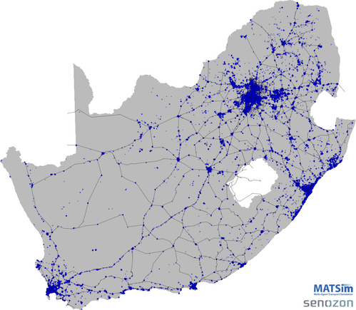
For each of the nine study areas, we limited the freight subpopulation to those vehicles that conduct at least one activity inside the envelope of the study area.

References:

Joubert, J.W., Axhausen, K.W. (2011). Inferring commercial vehicle activities in Gauteng, South Africa. Journal of Transport Geography, 19(1), 115-124.

Joubert, J.W., Axhausen, K.W. (2013). A complex network approach to understand commercial vehicle movement. Transportation, 40(3), 729–750.

Minnesota Population Centre (2013). Integrated Public Use Microdata Series, International: Version 6.2 (Machine-readable database). Minneapolis, University of Minnesota.

Müller, K., Axhausen, K.W. (2012). Multi-level fitting algorithms for population synthesis, Working paper, 821, Institute for Transport Planning and Systems (IVT), ETH Zurich, Switzerland.

R Core Team (2014). R: A language and environment for statistical computing. R Foundation for Statistical Computing, Vienna, Austria.

MATSim Community Space

Population generation